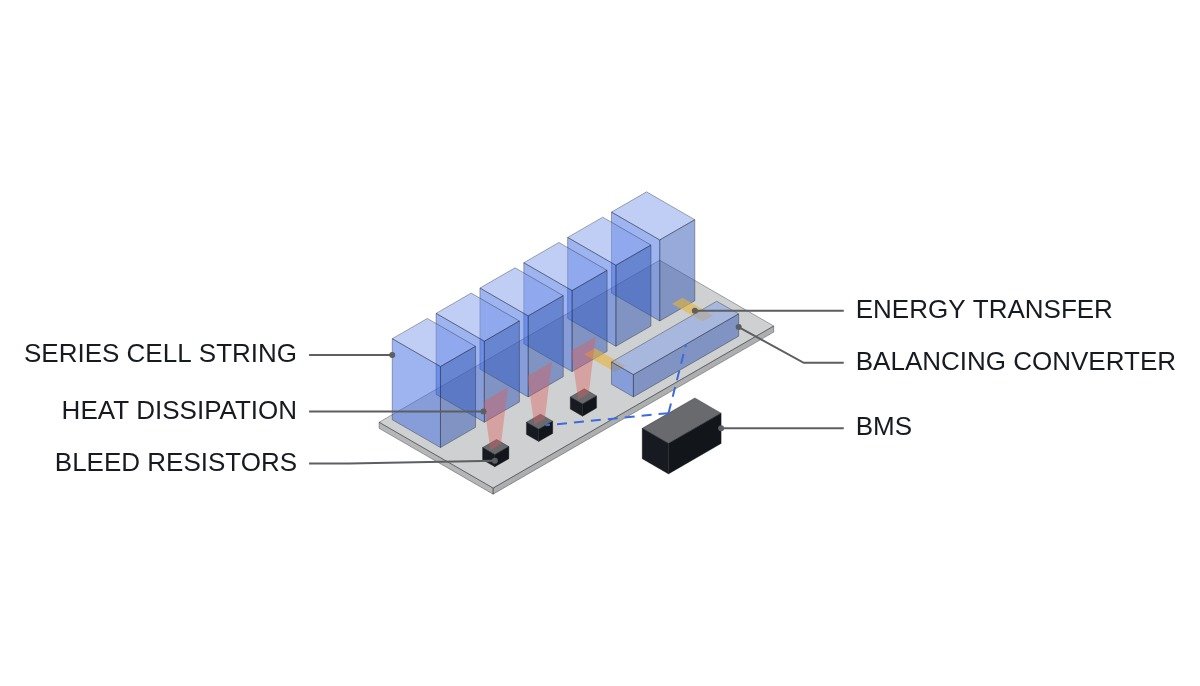
Bottom line first. Cell balancing does not add pack capacity; it pulls back state-of-charge (SOC) differences between cells. Passive balancing burns energy from high cells in resistors to match the low ones, so it cannot change the fact that usable pack capacity is tied to the cell with the smallest capacity. Active balancing moves energy between cells and can partly get past that limit, at the cost of more components and switching noise. A pack built from well-matched new cells is served fine by passive balancing; active balancing earns its place in packs with large cell-to-cell capacity spread, such as second-life packs and large ESS after years of operation.
Where it wins, where it doesn’t
Current condition
Many field complaints that “balancing isn’t working” come from lumping two causes into one. There are two kinds of cell-to-cell spread. One is SOC spread, created by differences in self-discharge rate. The other is capacity spread, created by differences in ageing rate. They look similar in voltage readings, but they call for different remedies.
After the change
Separate the causes and the choice becomes clear. SOC spread widens slowly over time, so a small, steady current is enough to pull it back, and passive balancing does this cheaply. Capacity spread is different: even if cells are aligned at the top of charge, the lowest-capacity cell reaches its discharge cut-off first at the bottom and stops the pack. Top-aligned passive balancing cannot fix that. Active balancing can move energy from stronger cells to the weak one during discharge and delay the point at which the weak cell hits cut-off.
Connecting logic
The decision therefore comes down to one question: is the pack bottleneck SOC spread or capacity spread? A pack assembled from new cells sorted by capacity grade starts with little capacity spread, and over its life the main component of spread is SOC. Packs rebuilt from second-life cells, or large racks with uneven temperature distribution, tend to be dominated by capacity spread. Match the method to the dominant component.
Method comparison
| Item | Passive | Active |
|---|---|---|
| Principle | Resistive discharge (dissipated as heat) | Energy transfer between cells or modules |
| Spread addressed | SOC spread | SOC spread plus part of capacity spread |
| Operating window | Mainly top of charge and rest | Charge, discharge and rest |
| Circuit | Resistor plus switch | Inductors, transformers, many switches |
| Heat | All balancing energy becomes heat | Only conversion losses become heat |
| Noise source | Negligible | Switching noise |
| Failure modes | Simple (resistor or switch open or short) | Many converter failure paths |
The key row is “spread addressed”. The only problem passive balancing cannot solve is capacity spread, and if that is not the pack bottleneck there is no reason to accept the part count and failure paths of an active system. Conversely, if capacity spread is the bottleneck, simply raising passive current adds heat and leaves usable capacity unchanged.
Required balancing current and heat
Balancing current is the amount of spread to be recovered divided by the time available for balancing. Assumptions: cell capacity 100Ah, 4 hours per day available for balancing, cell voltage 4.0V while passive balancing is active. A 1% spread is 1Ah, so the required current is 1Ah / 4h = 250mA.
| Daily spread (assumed) | Spread amount | Required current | Dissipation per cell |
|---|---|---|---|
| 0.2% | 0.2Ah | 50mA | 0.2W |
| 0.5% | 0.5Ah | 125mA | 0.5W |
| 1.0% | 1.0Ah | 250mA | 1.0W |
| 2.0% | 2.0Ah | 500mA | 2.0W |
Dissipation per cell is P = V x I = 4.0V x current. Getting 250mA needs a bleed resistor of 4.0V / 0.25A = 16Ω. If one board bleeds 12 channels at once, board heat is 12W at 1% spread and 24W at 2%. Because the current and heat needed to recover the same percentage spread scale with cell capacity, the limit of passive balancing in large-format cells shows up first as board heat, before it shows up as insufficient correction.
Time-sharing measurement and balancing
Apart from the choice of method, there is an electrical issue that is easy to miss. Where balancing current shares the cell voltage sense wires, current flowing through sense-wire and connector contact resistance creates a voltage drop that skews the cell voltage reading. If that error feeds back into the balancing decision, balancing may never stop, or the wrong cell gets discharged.
The usual cure is to split measurement and balancing in time: pause balancing for measurement and read the cell once its voltage has settled. Active systems are more sensitive to this because switching noise can couple into the measurement channels; the actual effect requires waveform analysis and field measurement.
When to decide which cell needs balancing matters as much as the method. Voltage difference reflects SOC difference accurately only in regions where cell voltage moves clearly with SOC. In cells such as LFP, whose voltage curve is flat through mid-SOC, a few mV difference there may be a large SOC gap or just measurement error. For such cells, select balancing targets only near the top of charge where the voltage slope steepens, and hold off in the flat region to avoid misoperation.
Decision sequence
- From operating history, separate whether cell voltage spread is large at the top of charge or at the bottom of discharge. If it opens only at the bottom, it is capacity spread.
- Quantify cell capacity spread with capacity tests or SOH estimation.
- If SOC spread dominates, compute the required current as above and keep passive balancing if board heat stays within limits.
- If capacity spread dominates and the economic value of recovered usable capacity exceeds the component cost, evaluate active balancing.
- If you adopt active balancing, measure the effect of switching noise on cell voltage sensing and communication lines on prototypes.
The most common mistake is skipping steps 1 and 2 and choosing a method first. Adding an active circuit before the cause of spread is separated raises cost with no way to confirm the effect. If the cause is confirmed as capacity spread, the rationale for active balancing is on record in numbers, which makes both the investment decision and later verification easier.
Boundary conditions
The advantage of active balancing disappears under some conditions. First, even with large capacity spread, if replacing the weak cell is cheaper, cell replacement beats an active circuit. Second, energy transfer has conversion losses, so in packs where little energy needs to move, the efficiency difference from passive balancing is negligible. Third, a fault in the active circuit itself can drive cells toward overcharge or overdischarge, so cell protection must sit on a voltage protection path independent of the balancing circuit, and the cost of providing that belongs in the comparison.
Fourth, in packs where temperature distribution is the root cause of spread, balancing only treats the symptom. If cells in one location always run hotter, they age faster and keep generating new capacity spread, and spread reopens whatever the balancing method. In that case, fix the coolant path and cell layout before changing the balancing circuit. The first step is to check in operating data whether the cells that drift are always in the same place.
The single selection rule: if what stops pack discharge is cell-to-cell capacity spread and moving energy is cheaper than replacing that cell, choose active; if the only cause is SOC spread, choose passive.