To state the conclusion first: wind and solar often peak at different times, both within the day and across seasons, so combining them flattens the combined output. But this complementarity turns into project revenue only when the two plants share the same grid connection capacity. Put both behind one point of connection and annual energy per kW of connection rises; connect them separately and the smoothing gain belongs to the grid as a whole while each owner keeps its own variability. And the degree of complementarity can be confirmed only by simultaneous measurement at the specific site, not by general rules.
Where It Wins, Where It Doesn’t
Under current conditions, a solar plant receives connection capacity sized to its maximum output. That capacity is full for only a few midday hours and empty in the morning, evening, and night. A wind plant is the same: connection capacity sized for strong winds sits idle in light winds. Where connection capacity is scarce, those idle hours are pure waste.
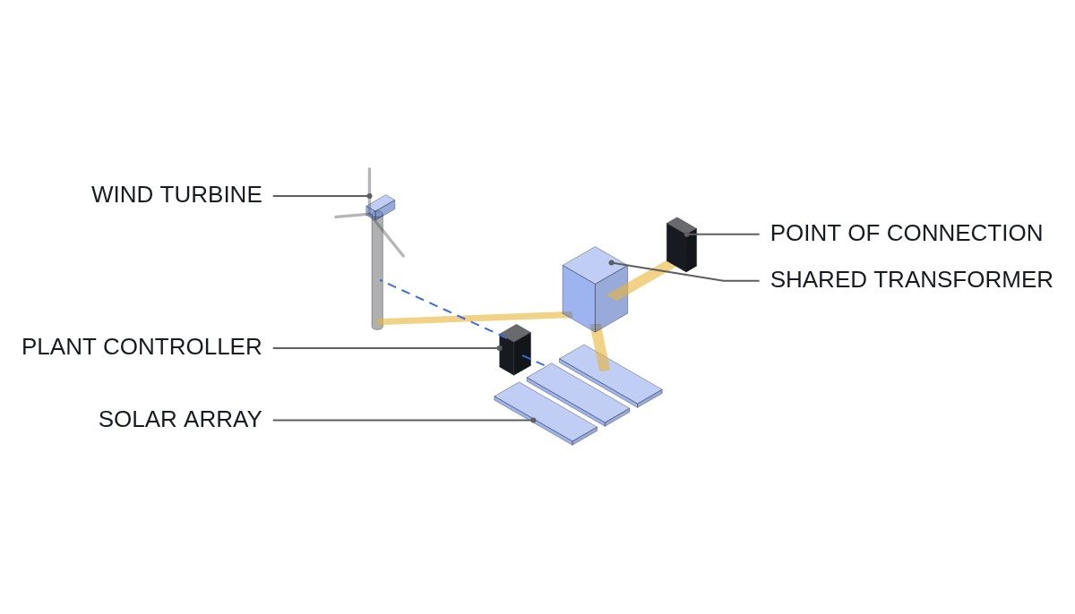
Combine the two behind the same connection point and things change. Wind uses the connection capacity at night and on cloudy days when solar rests, and solar uses it on clear midday hours with light wind. Even if the combined installed capacity exceeds the connection capacity, if the hours in which both hit maximum output together are short, the loss from limiting the excess is small. The result is more energy delivered through the same connection capacity.
The connecting logic is this. The economic value of complementarity arises when a scarce resource is shared. If that scarce resource is connection capacity, a transformer, or a transmission line, the two plants must actually share it for the gain to reach the owner. If nothing is shared, smoothing is good news for the grid operator but never appears on an individual project’s income statement.
Complementarity by Time Scale
Complementarity must be examined separately at each time scale. Within the day, solar concentrates at midday, while wind at some sites strengthens at night or early morning. Across seasons, in Korea wind speeds tend to be higher in winter under the northwesterly monsoon, while solar tends to produce most in spring and less in the summer rainy season. These tendencies vary with terrain and distance from the coast, however, so project decisions require simultaneous measured data from the site in question.
At the scale of weather events, complementarity can break down. When winds exceed a certain level, as in a typhoon, wind turbines shut down for protection (cut-out), and on the same day solar output falls under cloud. Conversely, on clear, windy spring days both plants run high at the same time. These simultaneous-maximum hours become the constraint on combined design.
| Time scale | Solar | Wind | Complementary? |
|---|---|---|---|
| Within the day | Midday peak | Site-dependent, some sites strong at night | Possible |
| Seasonal | More in spring, less in rainy season (tendency) | Stronger in winter (tendency) | Possible |
| Clear, windy day | High | High | Simultaneous max |
| Typhoon or storm | Low | Stopped at cut-out | Simultaneous low |
The top two rows show the gain from combining; the bottom two show its limits. Design must be sized to the limits, not the gain. Simultaneous-maximum hours set the loss from limiting output above connection capacity, and simultaneous-low hours set the gap that remains even after combining.
The Principle of Smoothing and the Connection-Capacity Calculation
The variability of the combined output is expressed as variance: Var(S + W) = Var(S) + Var(W) + 2 × Cov(S, W), where S is solar output and W is wind output. If the covariance of the two is negative, combined variability is smaller than the sum of the parts; if zero, they simply add; if positive, it actually grows. Complementarity is ultimately a question of the sign and size of that covariance.
The connection-capacity calculation works like this. Assumption: connection capacity C, solar capacity S_cap, wind capacity W_cap, with S_cap + W_cap > C. The excess is limited only in hours when the sum of the two outputs exceeds C, so the lost energy is the sum of max(0, S + W − C) over hourly simultaneous measured (or simultaneously simulated) data. Compare that value with the additional annual energy delivered by combining, and the appropriate combined size emerges.
The inputs to this calculation must be both outputs on the same time axis. Take monthly solar averages and monthly wind averages separately and add them, and the simultaneous-maximum hours are buried in the averages, underestimating the loss from limiting the excess.
There is also the option of shifting the excess into storage behind the connection point instead of discarding it. Storage capacity is then set by how long simultaneous maxima last, so at sites where they are short and frequent a small storage system suffices, while at sites where they run long the storage cost can exceed the combining gain.
Electrical Conditions for a Combined Plant
Sharing a connection point requires a power plant controller that limits the combined output of both plants at the point of connection. The controller reads the connection-point meter and splits output setpoints between the plants so the sum does not exceed connection capacity. The response speed of that command path and its behavior on loss of communication, namely whether each plant converges to a predefined safe output when communication drops, must be fixed at design stage.
Protection coordination also needs revisiting. Inverter-based solar and wind, which may carry rotating-machine characteristics depending on turbine type, contribute differently to fault current and behave differently during grid faults. Whether the connection-point relay settings suit both plants after combining must be confirmed by grid studies and requires waveform analysis and field measurement.
| Connection setup | Who gets the gain | Condition |
|---|---|---|
| Shared connection point | Owner (connection use) | Short simultaneous-max hours |
| Separate connections, same owner | Partial (joint forecasting and operation) | Integrated operation |
| Separate connections, different owners | Grid as a whole | No individual project gain |
What this table sums up is that for the same two plants, the owner of the complementarity gain changes with the connection setup. Before citing complementarity in a project review, first confirm that the setup matches the first row.
Decision Sequence
- Measure wind and irradiance simultaneously on the same time axis at the candidate site, or obtain simultaneous simulated data for the same period.
- Calculate the hourly correlation between the two outputs and the simultaneous-maximum hours.
- For each combination of installed capacity against connection capacity, calculate the excess-limiting loss and annual delivered energy.
- Decide the output-limiting method of the connection-point plant controller and the safe output on loss of communication.
- Confirm protection coordination after combining through grid studies.
Boundary Conditions
The complementarity gain disappears under two conditions. First, when the correlation between the two outputs comes out positive at the site. In terrain where wind strengthens on clear days, simultaneous-maximum hours grow long and combining only increases excess-limiting losses. Second, when the two plants sit on different connection points and share no equipment. Smoothing is then a gain for the grid as a whole, not a revenue basis for an individual project.
Conversely, at sites where connection capacity is scarce and the hours when one plant’s output is empty are clear, combining can be a faster alternative to securing new connection capacity.
The single decision criterion is this: combine wind and solar only at sites where they share the same connection point and simultaneously measured combined output exceeds connection capacity for only a short time.